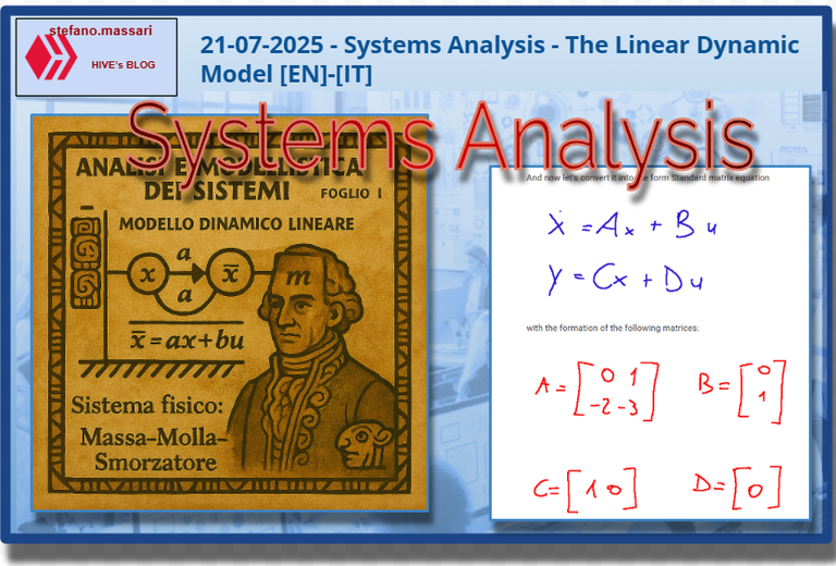
21-07-2025 - Systems Analysis - The Linear Dynamic Model [EN]-[IT]

~~~ La versione in italiano inizia subito dopo la versione in inglese ~~~

ENGLISH

21-07-2025 - Systems Analysis - The Linear Dynamic Model [EN]-[IT]
With this post, I'd like to provide a brief introduction to the topic mentioned above.
(code notes: X_85)

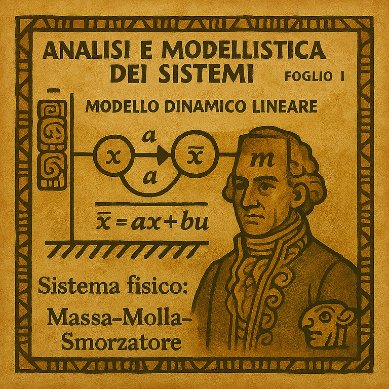
Image created with artificial intelligence, the software used is Microsoft Copilot

The Linear Dynamic Model

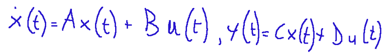
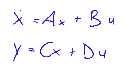
We talk about a linear dynamic model when we have a real system to analyze. Let me try to explain. Let's first imagine we have a real system in front of us, whether mechanical, electronic, or robotic. At this point, we want to analyze this system, and to do this, we can describe it with a linear model. The linear model is typically expressed in state-space form. What we see below is precisely this typical form.

WHERE:
A, B, C, D are constant matrices.

The advantages of having a linear dynamic model

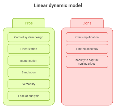
Image created with artificial intelligence, the software used is napkin.ai

We choose to translate a real-world model into a linear dynamic model for several reasons. These reasons include control system design, linearization of nonlinear systems, identification, simulation, versatility, and, above all, simplicity of analysis.

Dynamic parameters
To translate a real-world system into a linear dynamic model, we need to identify the dynamic parameters. As we said, we are analyzing a system that is subject to change, so we need to identify the physical constants that characterize its dynamic behavior. Let's try an example. Imagine having an anthropomorphic arm, that is, a robot with a mechanical arm. In this case, the physical constants that characterize the dynamic behavior of our robotic arm could be the masses, moments of inertia, and friction between the moving parts.
NOTE: The ability to reliably describe the behavior of many elements with a linear or linearized dynamic model allows us to characterize the dynamic behavior through some appropriately defined parameters. This is important to facilitate the analysis of a real system.

The Calculation Process
-1-
The calculation process begins with model construction. To build a model, we need to define the linear dynamic equations.
-2-
Next, we need to collect data through experimental measurements, recording the inputs and outputs.
-3-
The third step is the formation of the regression. Essentially, in this step, we try to connect the data to the parameters.
-4-
The calculation process concludes with the estimation of the parameters using several methods.

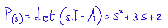
The Characteristic Polynomial

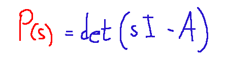
The characteristic polynomial of a linear dynamical system is shown above. It is usually expressed in matrix form (like the example above).

Where:
s = complex Laplace variable
I = identity matrix
A = state matrix of the system

This is sometimes also called the characteristic polynomial of matrix A, which is precisely the polynomial obtained by setting the equation det(aI-A)=0.

But what is it for?
The characteristic polynomial is used to understand the internal dynamics of a linear system. Once we've analyzed the characteristic polynomial, we can understand the system's stability, its response speed, and, if applicable, its oscillatory behavior.

Example
I'll try to quickly describe how to write a linear dynamics model. Please note, I won't go through all the steps, but my intention is to explain the purpose of translating a real system into a linear dynamics model.

Let's take a Mass-Spring-Damper system as an example.

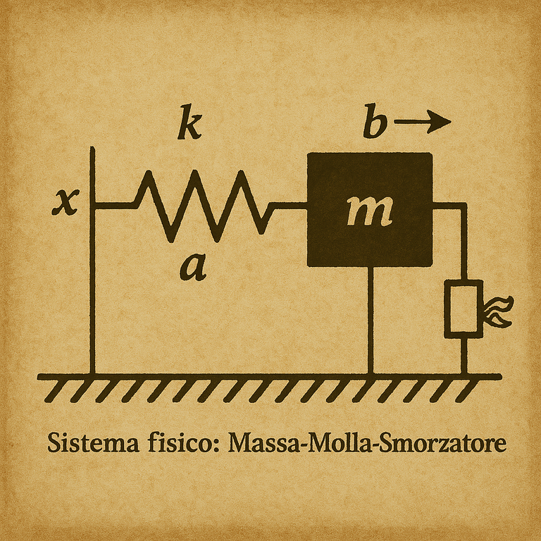
image created with artificial intelligence, the software used is Microsoft Copilot

Imagine a cart sliding on a horizontal guideway, connected to a spring with a viscous damper, and subjected to an input force.

Data summary:
One spring with spring constant K
One viscous damper with coefficient b
System subjected to an input force u(t)

The parameters are as follows:
Mass m = 1 kg
Spring constant k = 2 N/m
Damper b = 3 Ns/m
Input force = u(t)
Output y(t) = x(t)

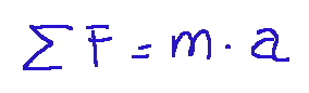
solution
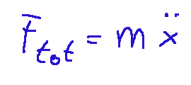
Remember Newton's second law!
image.png

... and apply it to the exercise in shape

We will have the following:

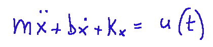
Substituting the numerical values, we obtain the following Formula

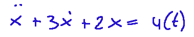
Here we are
and now we've reached the point of writing the state form and translating it all into a linear dynamic model.

We will therefore have the following system of equations:

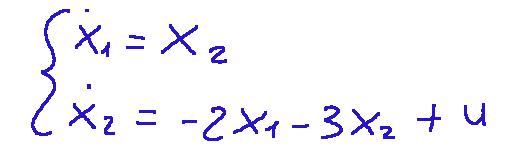
And now let's convert it into the form Standard matrix equation

with the formation of the following matrices:

Let's construct the polynomial Characteristic:

Result
At this point, we know that the result of the linear model is as follows:

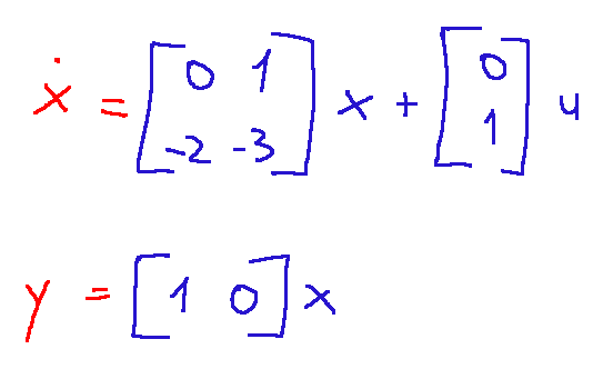
In this case, we have built a linear dynamic model for a mechanical system. Linearization consists of analyzing matrices A, B, C, and D.
Matrix A is the internal dynamics matrix of the system.
Matrix B shows how the input affects the system.
Matrix C is the system's output.

What does all this mean?
This analysis suggests that the position and velocity of the body change over time according to the linear equations of the system. It also suggests that the input force u(t) modifies the acceleration and that the output measures only one position.

Conclusions
A linear dynamic model is useful in engineering for various reasons, both theoretical and practical, and calculating this model allows us to identify the behavior of a system.

Question
The linear dynamic model was not invented by a single person, but is the result of many methodologies that were applied one after another and ultimately led to the creation of a method for constructing a linear dynamic model. Did you know that Pierre Simon Laplace (1749-1827), French mathematician and physicist, was one of the first to solve linear dynamical models in the complex domain using his famous Laplace transform?

ITALIAN

21-07-2025 - Analisi dei sistemi - Il modello dinamico lineare [EN]-[IT]
Con questo post vorrei dare una breve istruzione a riguardo dell’argomento citato in oggetto
(code notes: X_85)

immagine creata con l’intelligenza artificiale, il software usato è Microsoft Copilot

Il modello dinamico lineare

Parliamo di modello dinamico lineare quando davanti a noi abbiamo un sistema reale da analizzare. Provo a spiegarmi meglio. Immaginiamo, prima di tutto, di avere davanti a noi un sistema reale che può essere un sistema meccanico, elettronico oppure robotico.a questo punto vogliamo cercare di analizzare questo sistema e per fare questo possiamo descriverlo con un modello lineare. Il modello lineare è tipicamente espresso in forma state-space. Quello che vediamo qui sotto è proprio la forma tipica.

DOVE:
A, B, C, D sono matrici costanti.

I vantaggi di avere un modello lineare dinamico

immagine creata con l’intelligenza artificiale, il software usato è napkin.ai

Scegliamo di tradurre un modello reale in un modello lineare dinamico per diversi motivi. Questi motivi sono la progettazione di un sistema di controllo, la linearizzazione di sistemi non lineari, l’identificazione, la simulazione, la versatilità e soprattutto la semplicità di analisi.

Parametri dinamici
Per tradurre un sistema reale in un modello dinamico lineare abbiamo bisogno di identificare quali sono i parametri dinamici. Come abbiamo detto stiamo analizzando un sistema che è soggetto a cambiamenti, quindi dobbiamo rilevare quali sono le costanti fisiche che caratterizzano il comportamento dinamico. Proviamo a fare un esempio. Immaginiamo di avere un braccio antropomorfo, cioè un robot con un braccio meccanico. In questo caso le costanti fisiche che caratterizzano il comportamento dinamico del nostro braccio robotico possono essere le masse, i momenti di inerzia e le frizioni tra gli organi in movimento.
NOTA: La possibilità di descrivere in maniera affidabile il comportamento di molti elementi con un modello dinamico lineare o linearizzato consente di potere caratterizzare il comportamento dinamico attraverso alcuni parametri opportunamente definiti. Questo è importante per facilitare l'analisi di un sistema reale.

Il processo di calcolo
-1-
Il processo di calcolo parte dalla costruzione del modello. Per costruire un modello abbiamo bisogno di definire le equazioni dinamiche lineari.
-2-
Dopodiché dobbiamo raccogliere i dati tramite le misure sperimentali, rilevando gli ingressi e le uscite.
-3-
Il terzo passaggio è la formazione del regresso. Sostanzialmente in questo passaggio dobbiamo cercare di collegare i dati ai parametri.
-4-
Il processo di calcolo si chiude con la stima dei parametri tramite alcuni metodi.

Il polinomio caratteristico

Qui sopra è mostrato il polinomio caratteristico di un sistema dinamico lineare. La forma in cui è espresso, solitamente, è quella matriciale (come l'esempio proposto qui sopra)

Dove:
s = variabile complessa di Laplace
I = matrice identità
A = matrice dello stato del sistema

Questo a volte viene chiamato anche come il polinomio caratteristico della matrice A che è appunto il polinomio che si ottiene impostando l'equazione det(aI-A)=0.

Ma a cosa serve?
Il polinomio caratteristico serve per comprendere la dinamica interna di un sistema lineare. Una volta analizzato il polinomio caratteristico potremmo comprendere la stabilità del sistema, la velocità di risposta ed in caso l'avesse, anche il comportamento oscillatorio.

Esempio
Provo a descrivere velocemente la scrittura di un modello dinamico lineare. Attenzione non svolgerò tutti i passaggi, ma la mia intenzione è spiegare a cosa serve la traduzione di un sistema reale in un modello dinamico lineare.

Prendiamo come esempio un sistema Massa-Molla-Smorzante.

immagine creata con l’intelligenza artificiale, il software usato è Microsoft Copilot

Immaginiamo di avere un carrello che scorre su una guida orizzontale e collegato ad una molla con uno smorzatore viscoso e soggetto ad una forza d'ingresso.

Riepilogo dati:
n°1 molla con costante elastica K
n°1 uno smorzatore viscoso con coefficiente b
Sistema soggetto a una forza in ingresso u(t)

I parametri sono i seguenti:
Massa m = 1kg
Costante elastica k = 2N/m
Smorzatore b = 3 Ns/m
forza d'ingresso = u(t)
Uscita y(t) = x(t)

svolgimento
Ricordiamo la seconda legge di Newton

... e applichiamola all'esercizio nella forma

Avremo quanto segue:

sostituendo i valori numerici otterremo la seguente formula

Ci siamo
e adesso siamo arrivati al punto di scrivere la forma di stato e tradurre il tutto in un modello dinamico lineare

Avremo quindi il seguente sistema di equazioni:

ed ora passiamo a convertirlo nella forma matriciale standard

con la formazione delle seguenti matrici:

Costruiamo il polinomio caratteristico:

Risultato
A questo punto sappiamo che il risultato del modello lineare è il seguente:

In questo caso abbiamo costruito un modello dinamico lineare per un sistema meccanico. La linearizzazione consiste nell'analisi tra le matrici A,B,C e D.
La matrice A è la matrice dinamica interna del sistema
La matrice B mostra come l'ingresso agisce sul sistema
La matrice C è l'uscita del sistema

Tutto questo cosa significa?
Questa analisi ci suggerisce che la posizione e la velocità del corpo cambiano nel tempo seguendo ciò che dicono le equazioni lineari del sistema. Un'altra cosa che ci suggerisce è il fatto che la forza in ingresso u(t) modifica l'accelerazione e che l'uscita misura solo una posizione.

Conclusioni
Un modello lineare dinamico è utile in ingegneria per vari motivi, sia teorici che pratici ed il calcolo di questo modello ci permette di individuare il comportamento si un sistema

Domanda
Il modello dinamico lineare non è stato inventato da una singola persona, ma è il frutto di tante metodologie che si sono applicate una di seguito all'altra ed alla fine hanno permesso di creare un metodo per costruire un modello dinamico lineare. Lo sapevate che Pierre Simon Laplace (1749-1827), matematico e fisico francese, fu comunque uno tra i primi a risolvere modelli dinamici lineari nel dominio complesso tramite la sua celebre trasformata di Laplace?

THE END